 Written by: Jim Gilbert, CMTC Senior Consultant
The prior post stated that if a process is Capable and in Control, you will, by definition, get the outcome that the process was designed to produce. It is important to note that the phrase designed to produce means that we get what the process gives us but not necessarily what we want.
We want to understand how Six Sigma can help us ensure high product quality levels.
Let us use an example to help us better understand these important concepts. Let’s think about baking a loaf of bread. We have a list of ingredients (what they are and how much we need of each for a given batch which will also determine the weight of the loaf), a mixer, an oven and a bread pan.
A Process is transforming inputs into outputs. In our case, the ingredients are the Inputs. We also know that the oven needs to reach a given temperature for a specific amount of time with the dough inside.
Let’s assume that the oven is working correctly. It is Capable of producing what we want, a warm loaf of bread of a certain (specified) weight. Does the fact that the oven is working correctly guarantee that the bread will come out right? Of course not. What if the yeast is spent? This is an example of a Special Cause of variation: We are not getting the desired outcome because the process is out of Control. It is Capable, it will give us what we want when it is employed properly, but it is not in Control. In this case we have a faulty input, the yeast.
If we replace the bad yeast with new, good yeast, we will have brought the process back into Control. We now have a process that is both capable and in control and we can reasonably expect it to produce a good loaf of bread.
Process Capability is a measure of how capable the process is to produce the desired outcome, i.e. it can tell us what percentage of defects the process will inherently produce IF it is in Control.
If we have eliminated all Special Causes of variation as above, then the process is deemed in Control and all of the variation that we experience is variation that is inherent to the process itself. These include small variations in measured ingredients and slight variations in oven temperature. But the process is Robust enough to produce the desired outcome even with these sources of (inherent) variation.
Standard Deviation (Ϭ) is a measure of variation. It is calculated as the square root of the Variance. The reason that it is important to understand it this way is because of how we calculate it. We actually begin by calculating the Variance (Ϭ2) and then extract the square root of the Variance to provide us with the Standard Deviation.
The Empirical Rule is also known as the 68, 95, 99.7 Rule. This rule tells us that, for a Random Distribution [illustrated as a bell shaped curve similar to the one below], 68% of the observations will be within plus or minus 1 Standard Deviation, 95% of the observations will be within plus or minus 2 Standard Deviations and 99.7% of the observations will be within plus or minus 3 Standard Deviations.
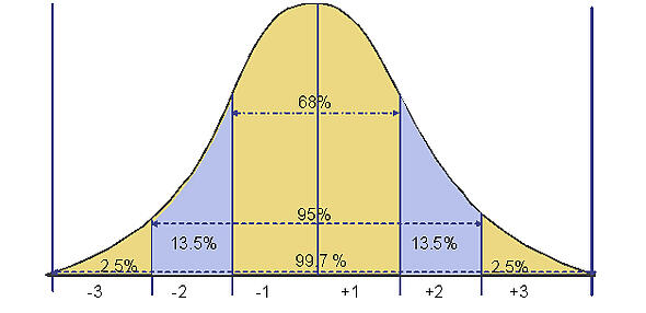
In the early 1920s Dr. William Shewhart, the Father of Quality, began developing Control Charts. He realized that if key process output variables (like the weight of a loaf of bread) were measured, and they created a distribution that would graph like the bell shaped curve above, then the variation being displayed was random and, therefore, inherent to the process. In other words, the process is behaving or operating in the manner it was designed to work. If the data is not random then there must be a logic to explain that behavior. That is what a Special Cause of Variation is.
Shewhart designed Control Charts like the ones below that include Control Limits. Control Limits (brown horizontal lines in graphs below)are usually a distance of plus or minus three Standard Deviations from the mean (green horizontal line). And, we know that if the data points are within the Contol Limits then our quality level is at least 99.7% good.
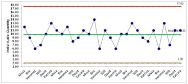 Statistical Process Control uses this knowledge to our advantage. Two graphs (run charts) are monitored by entering data and observing where the data points are located relative to the mean (average) and the Control Limits.
One chart, like the one above, is for plotting the average (X-bar) of the 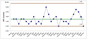 observations for each sample. The second chart, like the one below, is for plotting the range between the number of observations of the samples. As long as the plots fall within the Control Limits, and follow eight simple rules for randomness, then the process is deemed to be in Control. Please notice that there is no attention paid to the Specifications or Specification Limits (tolerances). A process that is in control is producing what it was designed (not necessarily intended) to produce. Thus, it may actually be producing bad outputs.
This issue is addressed in the next blog with a discussion on Process Capability.
Leave a Comment